Lux: Simulated Data and Underestimated Uncertainties

In this tutorial, we will build on our previous demonstration of Lux using simulated data to consider a case in which we are given data and uncertainties, but we believe the uncertainties are systematically underestimated for certain pixels. This issue sometimes appears in modeling stellar spectra, when telluric features, sky lines, or other issues are not fully accounted for in the uncertainties. We will demonstrate how to incorporate a (vector) parameter to handle this by adding an additional variance term to the likelihood, set by this parameter.

As usual, we will start with some standard imports and set up the simulated data.

import jax
import jax.numpy as jnp
import matplotlib.pyplot as plt
import numpy as np
import numpyro
import numpyro.distributions as dist

import pollux as plx
from pollux.models.transforms import FunctionTransform, LinearTransform

jax.config.update("jax_enable_x64", True)
%matplotlib inline

Generating simulated data

We will generate data for 2048 stars, with a latent dimensionality of 8, 2 labels, and 128 pixels in the spectra. We will follow the same prescription as in the previous tutorial to generate the simulated labels and spectra. After generating the data, we will then add in a systematic error (as a function of pixel number) that is not accounted for in the reported uncertainties.

from helpers import make_simulated_linear_data

n_stars = 2048  # number of simulated stars to generate in the train and test sets
n_latents = 8  # size of the latent vector per star
n_labels = 2  # number of labels to generate per star
n_flux = 128  # number of spectral flux pixels per star

rng = np.random.default_rng(seed=42)

A = np.zeros((n_labels, n_latents))
A[0, 0] = 1.0
A[1, 1] = 1.0

B = rng.normal(scale=0.1, size=(n_flux, n_latents))
B[:, 0] = B[:, 0] + 4 * np.exp(-0.5 * (np.arange(n_flux) - n_flux / 2) ** 2 / 5**2)
B[:, 1] = B[:, 1] + 2 * np.exp(-0.5 * (np.arange(n_flux) - n_flux / 4) ** 2 / 3**2)

data, truth = make_simulated_linear_data(
    n_stars=n_stars,
    n_latents=n_latents,
    n_flux=n_flux,
    n_labels=n_labels,
    A=A,
    B=B,
    rng=rng,
)

# Now we add a periodic systematic error to the flux:
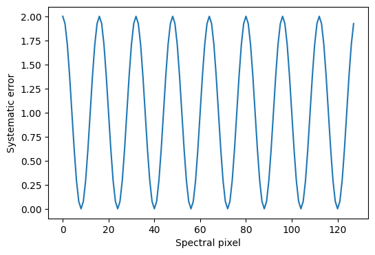
true_systematic_err = 2.0 * (np.cos(2 * np.pi * np.arange(n_flux) / (n_flux / 4))) ** 2
data["flux"] = rng.normal(data["flux"], scale=true_systematic_err)

The systematic error we add inflates the uncertainties significantly in a periodic pattern with pixel number:

plt.figure(figsize=(6, 4))
plt.plot(true_systematic_err)
plt.ylabel("Systematic error")
plt.xlabel("Spectral pixel")

Text(0.5, 0, 'Spectral pixel')

With simulated data in hand, we now proceed to run the Lux model on this data.

As with the previous tutorial, we will package this data (to prepare for using it in LuxModel) by defining a PolluxData instance with the data. We use the standard shift-and-scale normalization for the spectral flux data and labels (as shown in the previous tutorial):

all_data = plx.data.PolluxData(
    flux=plx.data.OutputData(
        data["flux"],
        err=data["flux_err"],
        preprocessor=plx.data.ShiftScalePreprocessor.from_data(data["flux"]),
    ),
    label=plx.data.OutputData(
        data["label"],
        err=data["label_err"],
        preprocessor=plx.data.ShiftScalePreprocessor.from_data(data["label"]),
    ),
)

preprocessed_data = all_data.preprocess()

For this example, we will again use the Lux model in a “supervised” or “train and apply” mode, in which we will train the model on a subset of the data and then apply it to the remaining data. We will use the first 1024 stars for training and the remaining 1024 stars for testing (since they are not ordered in any way):

train_data = preprocessed_data[: n_stars // 2]
test_data = preprocessed_data[n_stars // 2 :]
len(train_data), len(test_data)

(1024, 1024)

Constructing the Lux model

In our first demonstration, we will use the same Lux model as in the previous tutorial (i.e. without adding any additional parameters to learn the systematic error). We will then show that the model performs worse than a model that accounts for the (unknown) systematic error by simultaneously learning this vector.

Model 1: Lux without systematic error (same as in the previous tutorial)

model1 = plx.LuxModel(latent_size=8)
model1.register_output("label", LinearTransform(output_size=n_labels))
model1.register_output("flux", LinearTransform(output_size=n_flux))

opt_pars1, svi_results1 = model1.optimize(
    train_data,
    rng_key=jax.random.PRNGKey(112358),
    optimizer=numpyro.optim.Adam(1e-3),
    num_steps=32768,
    svi_run_kwargs={"progress_bar": False},
)
svi_results1.losses.block_until_ready()[-1]

Array(59929889.73705255, dtype=float64)

Let’s check the loss trajectory for the last 2000 steps to see if (visually) the optimization has converged:

plt.figure(figsize=(6, 4))
plt.plot(svi_results1.losses[-2000:])
plt.xlabel("Training epoch")
plt.ylabel("Loss")

Text(0, 0.5, 'Loss')

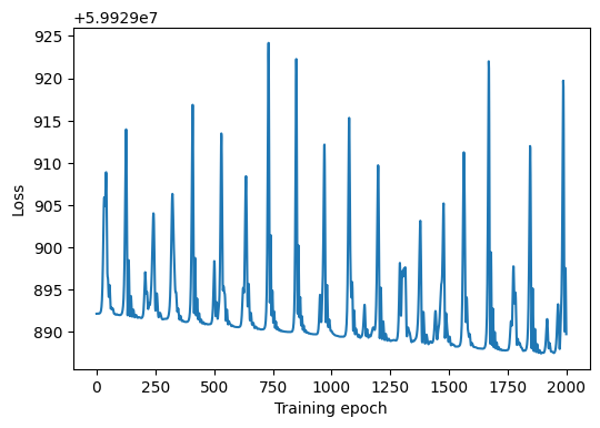
The loss function evolution looks approximately stable, so we will assume that the MAP optimization has converged. We can now evaluate the model on the test data and compare the results to the true labels.

fixed_pars1 = {
    "label": {"data": {"A": opt_pars1["label"]["data"]["A"]}},
    "flux": {"data": {"A": opt_pars1["flux"]["data"]["A"]}},
}

test_opt_pars1, test_svi_results1 = model1.optimize(
    test_data,
    rng_key=jax.random.PRNGKey(12345),
    optimizer=numpyro.optim.Adam(1e-3),
    num_steps=32_768,
    fixed_pars=fixed_pars1,
    svi_run_kwargs={"progress_bar": False},
)
test_svi_results1.losses.block_until_ready()[-1]

Array(68514528.82820797, dtype=float64)

predict_test_values1 = model1.predict_outputs(test_opt_pars1["latents"], fixed_pars1)

pt_style = {"ls": "none", "ms": 2.0, "alpha": 0.5, "marker": "o", "color": "k"}

fig, axes = plt.subplots(1, 2, figsize=(8, 4), layout="constrained")
for i in range(predict_test_values1["label"].shape[1]):
    axes[i].plot(
        predict_test_values1["label"][:, i], test_data["label"].data[:, i], **pt_style
    )
    axes[i].set(xlabel=f"Predicted label {i}", ylabel=f"True label {i}")
    axes[i].axline([0, 0], slope=1, color="tab:green", zorder=-100)
_ = fig.suptitle("Test set: predicted vs. true labels", fontsize=22)

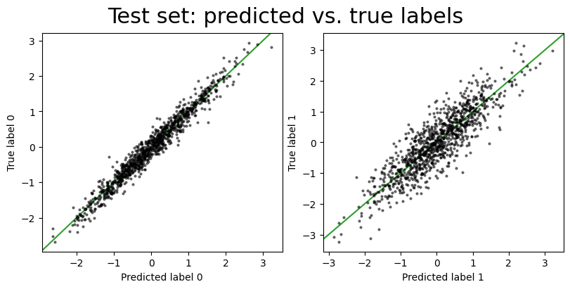
It looks like the model is doing a reasonable job of recovering the true labels, but the prediction error (variance) is large for the test set labels. We will now demonstrate how to improve this by adding a parameter to learn the systematic error.

Model 2: Lux with an inferred vector of extra flux uncertainties

We will now add a vector parameter to the model to learn the systematic error at each spectral pixel. We do this by specifying a custom LinearTransform instance with an additional parameter, s, to capture the systematic error. We will set the prior on this parameter to be a half-Normal distribution (a normal truncated at 0) with a mean of 0 and a standard deviation of 5 (i.e. we expect the systematic error to be small but allow the possibility of it being large).

err_trans = FunctionTransform(
    output_size=n_flux,
    transform=lambda err, s: jnp.sqrt(err**2 + s**2),
    param_priors={"s": dist.HalfNormal(5.0).expand((n_flux,))},
    param_shapes={},
)

We now define the model as we did before, but pass in the transform of the uncertainties we defined in the previous cell when defining the “flux” output:

model2 = plx.LuxModel(latent_size=8)
model2.register_output(
    "flux", LinearTransform(output_size=n_flux), err_transform=err_trans
)

# We register the label output as before, but we could have also added an unknown
# systematic uncertainty here
model2.register_output("label", LinearTransform(output_size=n_labels))

We now optimize as before:

opt_pars2, svi_results2 = model2.optimize(
    train_data,
    rng_key=jax.random.PRNGKey(112358),
    optimizer=numpyro.optim.Adam(1e-3),
    num_steps=32768,
    svi_run_kwargs={"progress_bar": False},
)
svi_results2.losses.block_until_ready()[-1]

Array(118697.24566318, dtype=float64)

And then optimize and evaluate the model on the test data:

fixed_pars2 = {
    "label": {"data": {"A": opt_pars2["label"]["data"]["A"]}},
    "flux": {
        "data": {"A": opt_pars2["flux"]["data"]["A"]},
        "err": {"s": opt_pars2["flux"]["err"]["s"]},
    },
}

test_opt_pars2, test_svi_results2 = model2.optimize(
    test_data,
    rng_key=jax.random.PRNGKey(12345),
    optimizer=numpyro.optim.Adam(1e-3),
    num_steps=32_768,
    fixed_pars=fixed_pars2,
    svi_run_kwargs={"progress_bar": False},
)
test_svi_results2.losses.block_until_ready()[-1]

Array(119841.51128579, dtype=float64)

predict_test_values2 = model2.predict_outputs(test_opt_pars2["latents"], fixed_pars2)

fig, axes = plt.subplots(1, 2, figsize=(8, 4), layout="constrained")
for i in range(predict_test_values2["label"].shape[1]):
    axes[i].plot(
        predict_test_values2["label"][:, i], test_data["label"].data[:, i], **pt_style
    )
    axes[i].set(xlabel=f"Predicted label {i}", ylabel=f"True label {i}")
    axes[i].axline([0, 0], slope=1, color="tab:green", zorder=-100)
_ = fig.suptitle("Test set: predicted vs. true labels", fontsize=22)

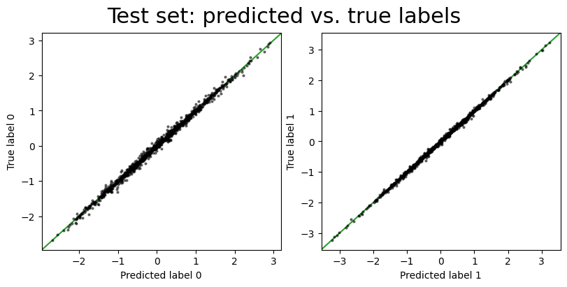
We can see visually here that the model with the systematic error parameter is doing a better job of recovering the true labels, with much less scatter in the predictions. We can also compare the loss function values for the two models:

test_svi_results1.losses[-1], test_svi_results2.losses[-1]

(Array(68514528.82820797, dtype=float64),
 Array(119841.51128579, dtype=float64))

The model with the systematic error parameter (model 2) has a much lower loss value (which, here, is related to the negative log-posterior probability of the model).

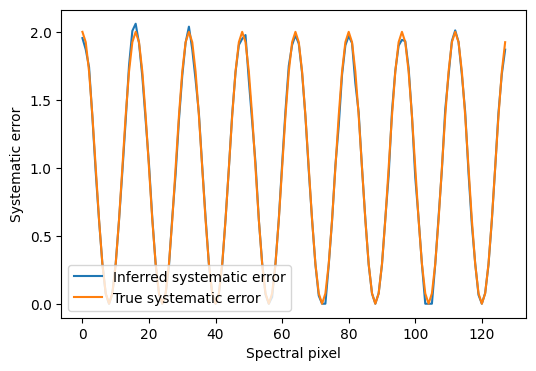
We can also compare the inferred systematic error parameter to the true systematic error:

inferred_s = all_data["flux"].preprocessor.inverse_transform_err(
    opt_pars2["flux"]["err"]["s"]
)

plt.figure(figsize=(6, 4))
plt.plot(inferred_s, label="Inferred systematic error")
plt.plot(true_systematic_err, label="True systematic error")
plt.xlabel("Spectral pixel")
plt.ylabel("Systematic error")
plt.legend(loc="lower left")

<matplotlib.legend.Legend at 0x7f6736c605c0>

To summarize, we have demonstrated how to incorporate a systematic error term into the Lux model to account for underestimated uncertainties in the data. We added a parameter to capture this for the spectral fluxes, per pixel. But we could have instead added a single value of the error inflation (i.e. for all pixels), or added a similar parameter for the label data. This can significantly improve the model’s ability to accurately predict label values, as demonstrated on simulated data.

More complex modifications of the models or additional parameters (e.g., adding a simultaneous model of the continuum flux shape) can also be incorporated, but that requires implementing a custom numpyro model. We will demonstrate this in a subsequent tutorial.