Lux: Getting Started 2 (Demo with APOGEE Data)

In this tutorial, we will build on the Getting Started 1 tutorial, which uses simulated data, to now demonstrate a Lux model applied to real data from the APOGEE survey (Data Release 17). For this test, we will use a subset of 1000 randomly-selected RGB stars with high signal-to-noise. We also sub-select the wavelength range to only keep one of the detector chips (the chip “a” or “red” in APOGEE lingo). This is a somewhat artificial use case in that we already have labels and spectra for all of these stars, but it allows us to demonstrate the use of Lux on real data and to explore how the model performs as we vary the number of latent dimensions.

We will start with some standard imports and then load and visualize the data.

import astropy.table as at
import h5py
import jax
import jax.numpy as jnp
import matplotlib.pyplot as plt
import numpy as np
import numpyro
import numpyro.distributions as dist
from astropy.stats import median_absolute_deviation as MAD

import pollux as plx
from pollux.models.transforms import LinearTransform

jax.config.update("jax_enable_x64", True)
%matplotlib inline

Load the data

We have pre-processed the data and stored it in an HDF5 file (available here) along with the corresponding rows from the APOGEE “allStar” catalog file.

with h5py.File("../_data/rgb-highSNR-1k-1chip.h5", "r") as f:
    apid = f["APSTAR_ID"][:]
    allstar = at.Table.read(f, path="allStar")
    assert np.all(allstar["APSTAR_ID"] == apid)

    all_wvln = f["wavelength"][:].astype("f8")
    all_flux = f["flux"][:].astype("f8")
    all_flux_err = f["flux_err"][:].astype("f8")

We now do some quality cuts on the spectral data. The flux data is a 2D array - one dimension corresponds to “stars” and the other “pixels” (wavelength):

all_flux.shape

(1000, 1980)

These are only minimal quality cuts because the stars have been pre-selected to have high signal-to-noise, so if you are working with a more heterogeneous APOGEE or other stellar spectral data set, you might need to do a more careful filtering. Here we require that the flux and flux error values are finite and that the error is positive. We also remove any pixels from the wavelength grid where >75% of stars have low SNR (which usually indicates bad pixels).

pix_snr = all_flux / all_flux_err

pixel_remove_mask = (
    # remove pixels that are the same for all stars (probably bad values)
    np.all(all_flux == all_flux[0], axis=0)
    # remove pixels where >75% of stars have low SNR (probably bad pixels)
    | ((pix_snr < 5).sum(axis=0) > 0.75 * pix_snr.shape[0])
)
flux = all_flux[:, ~pixel_remove_mask]
flux_err = all_flux_err[:, ~pixel_remove_mask]
wvln = all_wvln[~pixel_remove_mask]

# replace locations with zero or negative flux errors, or bad flux values:
bad_flux_mask = (all_flux_err <= 0) | (~np.isfinite(all_flux))
flux[bad_flux_mask] = 1.0
flux_err[bad_flux_mask] = 1e10  # set to large error to effectively ignore these pixels

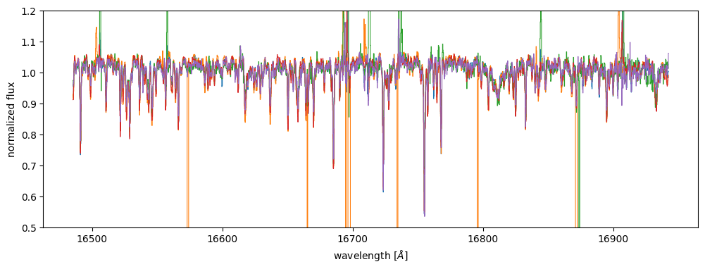
Let’s now visualize a few random spectra after this filtering:

rng = np.random.default_rng(123)
rand_idx = rng.choice(flux.shape[0], size=5, replace=False)

fig, ax = plt.subplots(figsize=(12, 4))
for i in rand_idx:
    _ = ax.plot(wvln, flux[i], marker="", drawstyle="steps-mid", lw=0.75)

_ = ax.set(xlabel=r"wavelength [$\AA$]", ylabel="normalized flux", ylim=(0.5, 1.2))

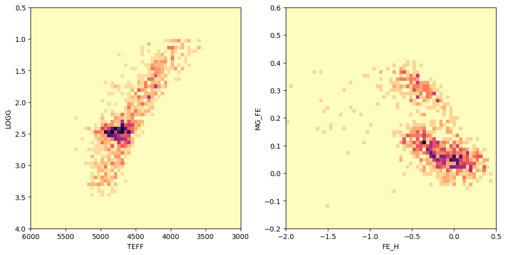
And here is a view of the label data (stellar parameters and abundances) for these stars:

fig, axes = plt.subplots(1, 2, figsize=(10, 5), layout="constrained")

axes[0].hist2d(
    allstar["TEFF"],
    allstar["LOGG"],
    bins=(np.linspace(3000, 6000, 64), np.linspace(0.5, 4.0, 64)),
    cmap="magma_r",
)
axes[0].set(xlim=(6000, 3000), ylim=(4.0, 0.5), xlabel="TEFF", ylabel="LOGG")

axes[1].hist2d(
    allstar["FE_H"],
    allstar["MG_FE"],
    bins=(np.linspace(-2.0, 0.5, 64), np.linspace(-0.2, 0.6, 64)),
    cmap="magma_r",
)
axes[1].set(xlim=(-2.0, 0.5), ylim=(-0.2, 0.6), xlabel="FE_H", ylabel="MG_FE")

[(-2.0, 0.5), (-0.2, 0.6), Text(0.5, 0, 'FE_H'), Text(0, 0.5, 'MG_FE')]

Assemble the data into Lux format

We now need to assemble the data into the format expected by Lux. The flux data is already in the form of a 2D array, but we need to convert the label data into a 2D array as well, where one dimension corresponds to “stars” and the other “labels”.

For the labels, we will use the stellar parameters (Teff, logg, [Fe/H]) and abundances of a few elements (Mg, C, N).

label_names = ["TEFF", "LOGG", "FE_H", "MG_FE", "C_FE", "N_FE"]
labels = np.array([allstar[name] for name in label_names]).T.astype("f8")
label_errs = np.array([allstar[f"{name}_ERR"] for name in label_names]).T.astype("f8")

all_data = plx.data.PolluxData(
    flux=plx.data.OutputData(
        flux,
        err=flux_err,
        preprocessor=plx.data.ShiftScalePreprocessor.from_data(flux),
    ),
    label=plx.data.OutputData(
        labels,
        err=label_errs,
        preprocessor=plx.data.ShiftScalePreprocessor.from_data(labels),
    ),
)

preprocessed_data = all_data.preprocess()
n_stars = len(all_data)
n_labels = len(label_names)
n_flux = len(wvln)
print(f"{n_stars=}, {n_labels=}, {n_flux=}")

n_stars=1000, n_labels=6, n_flux=1980

We now split the data into training and test sets using random indices:

idx = np.arange(n_stars)
rng.shuffle(idx)

train_idx = idx[: 3 * n_stars // 4]
test_idx = idx[3 * n_stars // 4 :]

test_data_unproc = all_data[test_idx]

train_data = preprocessed_data[train_idx]
test_data = preprocessed_data[test_idx]
len(train_data), len(test_data)

(750, 250)

We now pretend that we are missing label information for the test data:

test_flux_only = plx.data.PolluxData(flux=test_data["flux"])

Set up and train the Lux model

We are now ready to train and assess a Lux model. We will use the same architecture as in the Getting Started 1 tutorial, which is a bi-linear latent variable model with regularization / priors on the linear map matrix elements and the latent variables. However, similar to the “underestimated uncertainties” tutorial, we will also simultaneously infer a per-pixel “jitter” vector for the flux data. This is added in quadrature to the flux error values and allows the model to account for globally-underestimated uncertainties in the flux data, or for particularly bad pixels.

For this first demonstration, we will use a fixed number of latent parameters:

n_latents = 8 * n_labels

flux_err_trans = plx.models.transforms.FunctionTransform(
    output_size=n_flux,
    transform=lambda err, s: jnp.sqrt(err**2 + s**2),
    param_priors={"s": dist.HalfNormal(5.0).expand((n_flux,))},
    param_shapes={},
)
model = plx.LuxModel(latent_size=n_latents)
model.register_output("label", LinearTransform(output_size=n_labels))
model.register_output(
    "flux",
    LinearTransform(output_size=n_flux),
    err_transform=flux_err_trans,
)

We’re now set to train the model:

opt_pars, svi_results = model.optimize(
    train_data,
    num_steps=10_000,
    optimizer=numpyro.optim.Adam(1e-3),
    rng_key=jax.random.PRNGKey(42),
    svi_run_kwargs={"progress_bar": False},
)
loss = svi_results.losses.block_until_ready()

The training infers the optimal latent parameters for the training data, as well as the optimal values for the linear map matrices and the jitter vector for the flux data. We can now use these optimal parameters to predict labels for the test data. Like in the other tutorials, we do this by fixing the parameter values and inferring the latents for the test set given only the flux data:

fixed_pars = {
    "label": {"data": {"A": opt_pars["label"]["data"]["A"]}},
    "flux": {
        "data": {"A": opt_pars["flux"]["data"]["A"]},
        "err": {"s": opt_pars["flux"]["err"]["s"]},
    },
}

test_opt_res = model.optimize_iterative(
    test_flux_only, fixed_pars=fixed_pars, blocks=["latents"], progress=False
)
test_opt_pars = test_opt_res.params

Then, with inferred latent vectors for each star in the test set, we can predict the labels and “unprocess” the values (to put them back in unscaled values, i.e. with units like K for Teff, dex for logg, etc.):

predict_test_values = model.predict_outputs(test_opt_pars["latents"], fixed_pars)
predict_test_values = test_data.unprocess(predict_test_values)

Now we will compare the Lux-predicted labels for the test set with the “true” (i.e. APOGEE catalog values):

pt_style = {"ls": "none", "ms": 2.0, "alpha": 0.5, "marker": "o", "color": "k"}

fig, axes = plt.subplots(1, n_labels, figsize=(4 * n_labels, 4.5), layout="constrained")
for i in range(n_labels):
    axes[i].errorbar(
        predict_test_values["label"].data[:, i],
        test_data_unproc["label"].data[:, i],
        yerr=test_data_unproc["label"].err[:, i],
        **pt_style,
    )
    axes[i].set(xlabel=f"Lux {label_names[i]}", ylabel=f"ASPCAP {label_names[i]}")
    _val = np.median(test_data_unproc["label"].data[:, i])
    axes[i].axline([_val, _val], slope=1, color="tab:green", zorder=-100, alpha=0.5)

_ = fig.suptitle("Test set: Lux-predicted vs. APOGEE labels", fontsize=22)

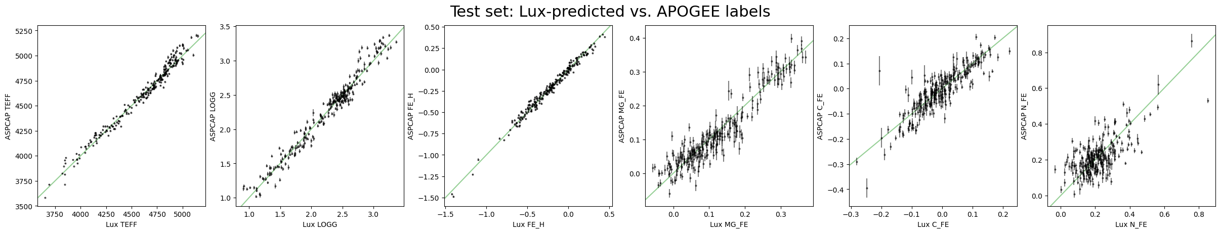
We see visually that the predicted labels match the true labels reasonably well, but there are some outliers. To get a quantitative measure of the prediction quality, we can also compute the root mean-square error (RMSE) and robust prediction scatter for each label:

resid = predict_test_values["label"].data - test_data_unproc["label"].data
err = test_data_unproc["label"].err

rmse = np.sqrt(np.mean(resid**2, axis=0))
mad_std = 1.5 * MAD(resid, axis=0)

for i in range(n_labels):
    print(
        f"{label_names[i]:>5s}: RMSE = {rmse[i]:.3f}, robust = {mad_std[i]:.3f}, median err = {np.median(err[:, i]):.3f}"
    )

 TEFF: RMSE = 49.916, robust = 46.903, median err = 8.494
 LOGG: RMSE = 0.108, robust = 0.096, median err = 0.025
 FE_H: RMSE = 0.039, robust = 0.038, median err = 0.008
MG_FE: RMSE = 0.035, robust = 0.032, median err = 0.012
 C_FE: RMSE = 0.045, robust = 0.035, median err = 0.014
 N_FE: RMSE = 0.083, robust = 0.078, median err = 0.017

So for example, the RMSE for Teff is about 50 K (and the robust scatter estimates are about comparable), but the median catalog uncertainty (for the test set) is only about 9 K. We see that the RMSE or scatter in the predicted labels is about 4–5 times larger than the typical catalog uncertainty, which suggests that the model may not be fully capturing all of the information in the spectra that is relevant for predicting the labels. On the other hand, the catalog uncertainties are likely underestimated, and use the full spectrum, so the fact that the RMSE is larger than the median catalog uncertainty is not necessarily a concern here. This can be a useful diagnostic to compare the performance of different models, or to identify labels that are not being well-predicted by the model.

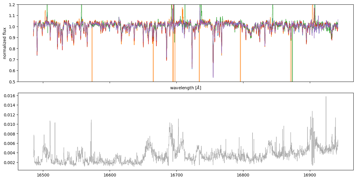
We can also look at the inferred “jitter” array to see if there are particular parts of the spectrum where the model needs to add more uncertainty to fit the data:

flux_s = opt_pars["flux"]["err"]["s"] * test_data["flux"].preprocessor.scale

rng = np.random.default_rng(123)
rand_idx = rng.choice(flux.shape[0], size=5, replace=False)

fig, axes = plt.subplots(2, 1, figsize=(12, 6), sharex=True, layout="constrained")
ax = axes[0]
for i in rand_idx:
    _ = ax.plot(wvln, flux[i], marker="", drawstyle="steps-mid", lw=0.75)

_ = ax.set(xlabel=r"wavelength [$\AA$]", ylabel="normalized flux", ylim=(0.5, 1.2))
ax = axes[1]
ax.plot(wvln, flux_s, marker="", drawstyle="steps-mid", lw=0.75, color="#aaaaaa")

[<matplotlib.lines.Line2D at 0x7fcd7ed46840>]

Varying the model hyperparameters

When training the model above, we fixed the number of latent parameters to 8 times the number of labels. This is an arbitrary choice (though we have found that this particular choice has worked well for our experiments with APOGEE data). A better approach for picking the number of latent parameters would be to use cross-validation. Below, we will experiment with varying the latent dimensionality to see how it affects the model performance.

We will train models with a range of choices for n_latents:

# Values of n_latents to explore.
n_latents_values = (n_labels * 2 ** np.arange(7)).astype(int)
print("n_latents values:", n_latents_values)

n_latents values: [  6  12  24  48  96 192 384]

all_results = {}
for n_latents in n_latents_values:
    # Construct the model with the same architecture and error model as before, but with
    # the new latent dimensionality:
    model = plx.LuxModel(latent_size=n_latents)
    model.register_output("label", LinearTransform(output_size=n_labels))
    model.register_output(
        "flux",
        LinearTransform(output_size=n_flux),
        err_transform=flux_err_trans,
    )

    # Optimize with the training data:
    opt_pars, _ = model.optimize(
        train_data,
        rng_key=jax.random.PRNGKey(12345),
        optimizer=numpyro.optim.Adam(5e-2),
        num_steps=2_000,
        svi_run_kwargs={"progress_bar": False},
    )

    # Optimize the latent parameters for the test set, keeping the output parameters
    # fixed to the values from training:
    fixed_pars = {
        "label": {"data": {"A": opt_pars["label"]["data"]["A"]}},
        "flux": {
            "data": {"A": opt_pars["flux"]["data"]["A"]},
            "err": {"s": opt_pars["flux"]["err"]["s"]},
        },
    }
    test_opt_res = model.optimize_iterative(
        test_flux_only, fixed_pars=fixed_pars, blocks=["latents"], progress=False
    )
    test_opt_pars = test_opt_res.params

    # Store the results for this model:
    all_results[n_latents] = {
        "model": model,
        "opt_pars": opt_pars,
        "fixed_pars": fixed_pars,
        "test_opt_pars": test_opt_pars,
    }

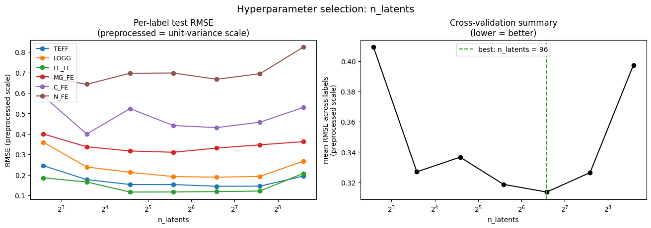
We use the mean RMSE of the preprocessed (unit-variance) data as our cross-validation summary statistic. Working in the preprocessed scale ensures that all labels contribute equally regardless of their natural units or dynamic range. Without this, the summary would be dominated by TEFF (in Kelvin) at the expense of abundance labels (in dex).

Note that because the “true” catalog labels themselves have uncertainties, the RMSE has an irreducible floor: even a perfect model should show nonzero RMSE. This floor doesn’t affect which value of n_latents is optimal, but it means the absolute RMSE values should not be interpreted as pure model error.

Once the RMSE curve has flattened or begins to turn over, i.e. adding more latent dimensions no longer improves predictions, there is no benefit to increasing n_latents. The best n_latents is where the mean RMSE is minimium:

all_rmse = []
for n_latents, res in all_results.items():
    model = res["model"]
    predict_test = model.predict_outputs(
        res["test_opt_pars"]["latents"], res["fixed_pars"]
    )
    resid = predict_test["label"] - test_data["label"].data
    all_rmse.append(np.sqrt(np.mean(resid**2, axis=0)))

    all_results[n_latents]["predict_test_unproc"] = test_data.unprocess(predict_test)

all_rmse = np.array(all_rmse)

mean_rmse = np.mean(all_rmse, axis=1)
best_idx = np.argmin(mean_rmse)
best_n_latents = n_latents_values[best_idx]

fig, axes = plt.subplots(1, 2, figsize=(13, 4.5), layout="constrained")

# Left: per-label RMSE (preprocessed scale)
for i, name in enumerate(label_names):
    axes[0].plot(n_latents_values, all_rmse[:, i], marker="o", label=name)
axes[0].set(
    xlabel="n_latents",
    ylabel="RMSE (preprocessed scale)",
    title="Per-label test RMSE\n(preprocessed = unit-variance scale)",
)
axes[0].set_xscale("log", base=2)
axes[0].legend(fontsize=9, loc="upper left")

# Right: mean RMSE across labels — the cross-validation summary statistic
axes[1].plot(n_latents_values, mean_rmse, marker="o", color="k")
axes[1].axvline(
    best_n_latents,
    color="tab:green",
    ls="--",
    lw=1.5,
    label=f"best: n_latents = {best_n_latents}",
)
axes[1].set(
    xlabel="n_latents",
    ylabel="mean RMSE across labels\n(preprocessed scale)",
    title="Cross-validation summary\n(lower = better)",
)
axes[1].set_xscale("log", base=2)
axes[1].legend(loc="upper center")

_ = fig.suptitle("Hyperparameter selection: n_latents", fontsize=14)

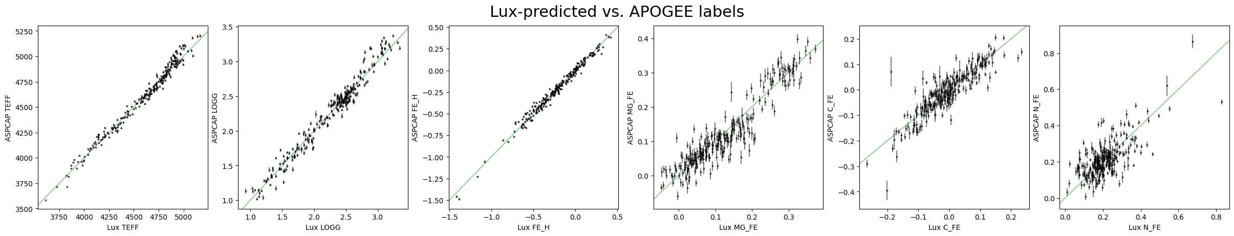
Let’s now visualize the results for the best value of n_latents:

fig, axes = plt.subplots(1, n_labels, figsize=(4 * n_labels, 4.5), layout="constrained")
for i in range(n_labels):
    predict_test_values = all_results[best_n_latents]["predict_test_unproc"]
    axes[i].errorbar(
        predict_test_values["label"].data[:, i],
        test_data_unproc["label"].data[:, i],
        yerr=test_data_unproc["label"].err[:, i],
        **pt_style,
    )
    axes[i].set(xlabel=f"Lux {label_names[i]}", ylabel=f"ASPCAP {label_names[i]}")
    _val = np.median(test_data_unproc["label"].data[:, i])
    axes[i].axline([_val, _val], slope=1, color="tab:green", zorder=-100, alpha=0.5)

_ = fig.suptitle("Lux-predicted vs. APOGEE labels", fontsize=22)

predict_labels = {
    k: predict_test_values["label"].data[:, i] for i, k in enumerate(label_names)
}

fig, axes = plt.subplots(1, 2, figsize=(10, 5), layout="constrained")

axes[0].hist2d(
    allstar["TEFF"],
    allstar["LOGG"],
    bins=(np.linspace(3000, 6000, 64), np.linspace(0.5, 4.0, 64)),
    cmap="magma_r",
)
axes[0].scatter(
    predict_labels["TEFF"],
    predict_labels["LOGG"],
    marker="o",
    color="tab:blue",
    s=4,
    label="Lux predictions",
)
axes[0].set(xlim=(6000, 3000), ylim=(4.0, 0.5), xlabel="TEFF", ylabel="LOGG")

axes[1].hist2d(
    allstar["FE_H"],
    allstar["MG_FE"],
    bins=(np.linspace(-2.0, 0.5, 64), np.linspace(-0.2, 0.6, 64)),
    cmap="magma_r",
)
axes[1].scatter(
    predict_labels["FE_H"],
    predict_labels["MG_FE"],
    marker="o",
    color="tab:blue",
    s=4,
    label="Lux predictions",
)
axes[1].legend(loc="upper left")
axes[1].set(xlim=(-2.0, 0.5), ylim=(-0.2, 0.6), xlabel="FE_H", ylabel="MG_FE")

[(-2.0, 0.5), (-0.2, 0.6), Text(0.5, 0, 'FE_H'), Text(0, 0.5, 'MG_FE')]

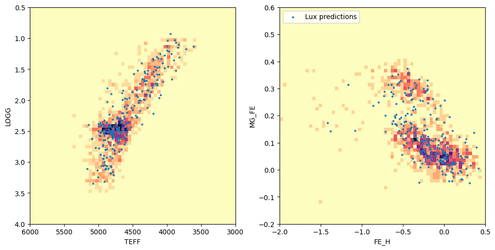
Nice, so the predicted labels capture the structure we expect to see in the stellar parameters and abundances.