Lux: Iterative Optimization for Linear Models

This tutorial demonstrates the optimize_iterative() method, which provides an efficient alternating optimization agenda for Lux models with linear transforms. This method exploits the linear structure of the model to solve sub-problems exactly using weighted least squares, often converging faster than gradient-based optimization with Adam (the default for optimize()).

This tutorial builds on the Getting Started tutorial, so we’ll skip the basic introductions and jump straight to comparing the two optimization approaches.

We’ll start with the standard imports:

import time

import jax
import matplotlib.pyplot as plt
import numpy as np
import numpyro
from helpers import make_simulated_linear_data

import pollux as plx
from pollux.models import LinearTransform

jax.config.update("jax_enable_x64", True)
%matplotlib inline

Generating simulated data

We’ll generate the same simulated data as in the Getting Started tutorial:

n_stars = 2048
n_latents = 8
n_labels = 2
n_flux = 128

rng = np.random.default_rng(seed=8675309)

A = np.zeros((n_labels, n_latents))
A[0, 0] = 1.0
A[1, 1] = 1.0

B = rng.normal(scale=0.1, size=(n_flux, n_latents))
B[:, 0] = B[:, 0] + 4 * np.exp(-0.5 * (np.arange(n_flux) - n_flux / 2) ** 2 / 5**2)
B[:, 1] = B[:, 1] + 2 * np.exp(-0.5 * (np.arange(n_flux) - n_flux / 4) ** 2 / 3**2)

data, truth = make_simulated_linear_data(
    n_stars=n_stars,
    n_latents=n_latents,
    n_flux=n_flux,
    n_labels=n_labels,
    A=A,
    B=B,
    rng=rng,
)

Package the data with preprocessors and create train/test splits:

all_data = plx.data.PolluxData(
    flux=plx.data.OutputData(
        data["flux"],
        err=data["flux_err"],
        preprocessor=plx.data.ShiftScalePreprocessor.from_data(data["flux"]),
    ),
    label=plx.data.OutputData(
        data["label"],
        err=data["label_err"],
        preprocessor=plx.data.ShiftScalePreprocessor.from_data(data["label"]),
    ),
)

preprocessed_data = all_data.preprocess()
train_data = preprocessed_data[: n_stars // 2]
test_data = preprocessed_data[n_stars // 2 :]

Setting up the model

We create a Lux model with two linear outputs, exactly as in the Getting Started tutorial:

model = plx.LuxModel(latent_size=n_latents)
model.register_output("label", LinearTransform(output_size=n_labels))
model.register_output("flux", LinearTransform(output_size=n_flux))

Comparing optimization methods

Now we’ll compare the standard optimize() method with the new optimize_iterative() function.

Standard optimization with optimize()

The standard approach uses gradient-based optimization (SVI with Adam) to jointly optimize all parameters:

t0 = time.time()
opt_pars_svi, svi_results = model.optimize(
    train_data,
    rng_key=jax.random.PRNGKey(112358),
    optimizer=numpyro.optim.Adam(1e-3),
    num_steps=10_000,
    svi_run_kwargs={"progress_bar": False},
)
svi_results.losses.block_until_ready()
svi_time = time.time() - t0
print(f"SVI optimization time: {svi_time:.2f} seconds")

SVI optimization time: 9.90 seconds

Iterative optimization with optimize_iterative()

The iterative approach exploits the linear structure of the model. For linear transforms like y = A @ z, the optimal latents (z) given A, and the optimal A given z, can each be solved exactly using weighted least squares. The algorithm alternates between these two steps:

1. Fix output parameters, solve for latents: Given the current A matrices, solve for optimal z using least squares

2. Fix latents, solve for output parameters: Given the current z, solve for optimal A matrices using least squares

This is repeated until convergence:

t0 = time.time()
iterative_result = model.optimize_iterative(
    train_data,
    max_cycles=50,
    tol=1e-6,
    rng_key=jax.random.PRNGKey(112358),
    progress=False,
)
iterative_time = time.time() - t0
print(f"Iterative optimization time: {iterative_time:.2f} seconds")
print(
    f"Converged: {iterative_result.converged} after {iterative_result.n_cycles} cycles"
)

Iterative optimization time: 3.13 seconds
Converged: True after 11 cycles

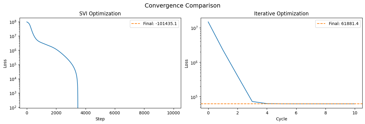
Comparing convergence

Let’s visualize how the loss evolves for both methods:

fig, axes = plt.subplots(1, 2, figsize=(12, 4), layout="constrained")

# SVI loss trajectory
axes[0].semilogy(svi_results.losses)
axes[0].set(xlabel="Step", ylabel="Loss", title="SVI Optimization")
axes[0].axhline(
    svi_results.losses[-1],
    color="tab:orange",
    ls="--",
    label=f"Final: {svi_results.losses[-1]:.1f}",
)
axes[0].legend()

# Iterative loss trajectory
axes[1].semilogy(iterative_result.losses_per_cycle)
axes[1].set(xlabel="Cycle", ylabel="Loss", title="Iterative Optimization")
axes[1].axhline(
    iterative_result.losses_per_cycle[-1],
    color="tab:orange",
    ls="--",
    label=f"Final: {iterative_result.losses_per_cycle[-1]:.1f}",
)
axes[1].legend()

plt.suptitle("Convergence Comparison", fontsize=14)

Text(0.5, 0.98, 'Convergence Comparison')

Evaluating on the test set

To evaluate the model on unseen data, we infer latents for the test set while keeping the trained model parameters fixed. We start with the SVI-trained parameters:

# Create fixed_pars containing the trained model parameters (everything except latents)
fixed_pars_svi = {k: v for k, v in opt_pars_svi.items() if k != "latents"}

# Create test data with only flux (we want to predict labels using only flux)
test_flux_only = plx.data.PolluxData(flux=test_data["flux"])

# Optimize latents for test set using SVI (fix model parameters)
# Use names=["flux"] to only model the flux output (since we don't have label data)
test_pars_svi, _ = model.optimize(
    test_flux_only,
    rng_key=jax.random.PRNGKey(42),
    optimizer=numpyro.optim.Adam(1e-3),
    num_steps=2000,
    fixed_pars=fixed_pars_svi,
    names=["flux"],
    svi_run_kwargs={"progress_bar": False},
)
# Merge the fixed parameters back with the optimized latents
test_pars_svi = {**fixed_pars_svi, **test_pars_svi}

Now we do the same for the iterative method. We can use blocks=["latents"] with fixed_pars to optimize only the latents while fixing the trained output parameters — no need to construct ParameterBlock instances or manually merge parameters afterward:

opt_pars_iter = iterative_result.params
fixed_pars_iter = {k: v for k, v in opt_pars_iter.items() if k != "latents"}

# Optimize latents for test set using iterative method.
# blocks=["latents"] restricts optimization to latents only; fixed_pars holds
# the trained output parameters fixed. result.params contains everything.
test_result_iter = model.optimize_iterative(
    test_flux_only,
    blocks=["latents"],
    fixed_pars=fixed_pars_iter,
    max_cycles=50,
    tol=1e-6,
    progress=False,
)
test_pars_iter = test_result_iter.params

# Predictions on test set from both methods
pred_svi = model.predict_outputs(test_pars_svi["latents"], test_pars_svi)
pred_iter = model.predict_outputs(test_pars_iter["latents"], test_pars_iter)

pt_style = {"ls": "none", "ms": 2.0, "alpha": 0.5, "marker": "o", "color": "k"}

fig, axes = plt.subplots(2, 2, figsize=(10, 10), layout="constrained")

# Top row: SVI predictions vs true
for i in range(2):
    axes[0, i].plot(pred_svi["label"][:, i], test_data["label"].data[:, i], **pt_style)
    axes[0, i].set(xlabel=f"Predicted label {i}", ylabel=f"True label {i}")
    axes[0, i].axline([0, 0], slope=1, color="tab:green", zorder=-100)
axes[0, 0].set_title("SVI: Label 0")
axes[0, 1].set_title("SVI: Label 1")

# Bottom row: Iterative predictions vs true
for i in range(2):
    axes[1, i].plot(pred_iter["label"][:, i], test_data["label"].data[:, i], **pt_style)
    axes[1, i].set(xlabel=f"Predicted label {i}", ylabel=f"True label {i}")
    axes[1, i].axline([0, 0], slope=1, color="tab:green", zorder=-100)
axes[1, 0].set_title("Iterative: Label 0")
axes[1, 1].set_title("Iterative: Label 1")

fig.suptitle("Test Set: Predicted vs. True Labels", fontsize=16)

Text(0.5, 0.98, 'Test Set: Predicted vs. True Labels')

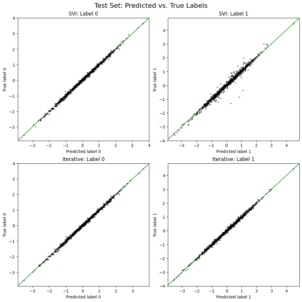
Both the SVI and iterative methods visually seem to predict the test set labels, but the iterative optimization appears to yield slightly better accuracy for this toy example.

Here’s another way to look at the test set prediction accuracy:

# Compute prediction errors on test set
svi_label_rmse = np.sqrt(np.mean((pred_svi["label"] - test_data["label"].data) ** 2))
iter_label_rmse = np.sqrt(np.mean((pred_iter["label"] - test_data["label"].data) ** 2))

svi_flux_rmse = np.sqrt(np.mean((pred_svi["flux"] - test_data["flux"].data) ** 2))
iter_flux_rmse = np.sqrt(np.mean((pred_iter["flux"] - test_data["flux"].data) ** 2))

print("Test Set Performance Comparison")
print("=" * 50)
print(f"{'Method':<20} {'Time (s)':<12} {'Label RMSE':<15} {'Flux RMSE':<15}")
print("-" * 50)
print(
    f"{'SVI (10k steps)':<20} {svi_time:<12.2f} {svi_label_rmse:<15.4f} {svi_flux_rmse:<15.4f}"
)
print(
    f"{'Iterative':<20} {iterative_time:<12.2f} {iter_label_rmse:<15.4f} {iter_flux_rmse:<15.4f}"
)

Test Set Performance Comparison
==================================================
Method               Time (s)     Label RMSE      Flux RMSE      
--------------------------------------------------
SVI (10k steps)      9.90         0.1127          0.4638         
Iterative            3.13         0.0593          0.2046         

When to use iterative optimization

The iterative optimization approach works well when your model is purely linear and should out-perform gradient-based methods in terms of speed, convergence, and often on prediction accuracy as well, given the closed-form solutions available for linear least squares problems.

For models with non-linear transforms (e.g., neural networks, Gaussian processes), you should use the standard optimize() method with gradient-based optimization.